![]()
25. Logistic regression#
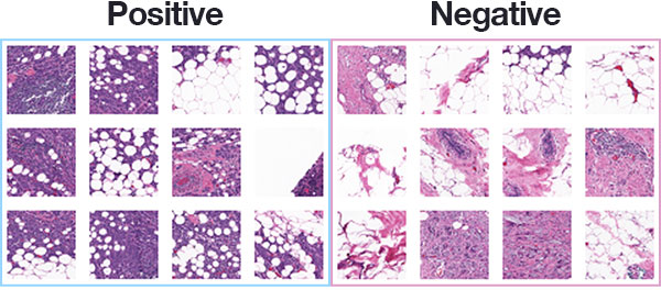
In previous classes we have used exploratory approaches to visualize and quantify relationships between variables. We used linear regression to make predictions about numeric values (e.g., boston house prices), now we will use logistic regression models for a classification problem. Here we will try and distinguish tissue samples as positive/negative for breast cancer.
Let’s load in our growing list of python packages that we are getting used to using.
import sklearn as sk
from sklearn.model_selection import train_test_split

import pandas as pd
import seaborn as sns
import matplotlib.pyplot as plt

import statsmodels.api as sm
import statsmodels.formula.api as smf
Then let’s load in the breast cancer dataset, and get it into a format we can use.
# The tissue sample dataset
df_cancer = ?

#take a look
?
25.1. Understand the data #
What kinds of data is the cancer data?
?
Are there missing values anywhere?
?
25.2. Visualize and Explore #
Histogram of the target variable
?
Plot the target variable (benign) on the y-axis with another variable on the x-axis. Try out a few different variables on the x-axis.
?
Create a heat map to help you explore
?
25.3. Data wrangling #
Data preprocessing (binary variables)
from sklearn.preprocessing import OrdinalEncoder

#get the columns names of features you'd like to turn into 0/1
bin_names = ['benign']

#create a dataframe of those features
bin_features = df_cancer[bin_names]

#fit the scaler to those data
bin_scaler = OrdinalEncoder().fit(bin_features.values)

#use the scaler to transform your data
bin_features = bin_scaler.transform(bin_features.values)

#put these scaled features back into your transformed features dataframe
df_cancer[bin_names] = bin_features

#take a look
df_cancer
bin_scaler.categories_
Data preprocessing (categorical variables)
Technician ID number is a categorical value, but it is being treated as a number (int64). Let’s convert it to a category.
df_cancer['technician'] = df_cancer.technician.astype('category')
#categorical variables
cat_names = ['technician']

#create dummy variables
df_cat = pd.get_dummies(df_cancer[cat_names])

#add them back to the original dataframe
df_cancer = pd.concat([df_cancer,df_cat], axis=1)

#remove the old columns
df_cancer = df_cancer.drop(cat_names, axis=1)

#take a look
df_cancer
Split our dataframe into training and testing datasets
#split the data into training and testing (80/20 split)
df_train, df_test = sk.model_selection.train_test_split(df_cancer, test_size=0.20)
#take a look training dataset
df_train.shape
#take a look
df_test.shape
Data pre-processing (numeric)
#Feature Scaling (after spliting the data!)
from sklearn.preprocessing import StandardScaler

#numeric variables
numb_names = df_train.drop(['benign','technician_1','technician_2','technician_3','technician_4'],axis=1).select_dtypes('number').columns.tolist()

#create the standard scaler object
sc = StandardScaler()

#use this object to fit (i.e., to calculate the mean and sd of each variable in the training data) and then to transform the training data
df_train[numb_names] = sc.fit_transform(df_train[numb_names])

#use the fit from the training data to transform the test data
df_test[numb_names] = sc.transform(df_test[numb_names])
25.4. Modeling and Prediction#
Let’s look building our second kind of model – logistic regression! How well can we predict the benign cases? This is similar to clustering analysis except we have the labels! Can we train a model to make the right predictions?
We will follow a general approach when building models. We will divide the dataset into training and testing datasets.
This lets us fit the model to one part of the data and then use the withheld data to test the predictions of the model. This helps us avoid overfitting our model!
Fit a model

Below choose a variable to predict if the tissue sample is benign or not.
In general when using sklearn to fit a model we will follow these steps:
#define model parameters
log_reg = smf.logit('benign ~ ?', data=df_train)

#fit the model to the training data
results = log_reg.fit()

#Get a summary of the model parameters
print(results.summary())
Visualize and explore the model predictions
Let’s look at where the model to a good/bad job of classifying images into benign or not!
#let's first predict values in the testing dataset
df_test['benign_prob'] = results.predict(df_test).round(2)

df_test['benign_pred'] = (df_test['benign_prob']>0.5).astype(int) #here we've used 0.5 as the threshold of benign or not!

df_test
Let’s plot the predicted and observed points!
sns.scatterplot(data=df_test,x='mean_symmetry', y='benign')
sns.scatterplot(data=df_test,x='mean_symmetry', y='benign')
sns.scatterplot(data=df_test,x='mean_symmetry', y='benign_pred')

How good is the model at classifying?
#confusion table
confusion_matrix = sk.metrics.confusion_matrix(df_test['benign'], df_test['benign_pred'])
print(confusion_matrix)
#more visual approach
sns.heatmap(confusion_matrix, annot=True)
plt.xlabel('Predicted label')
plt.ylabel('True label')
Measuring classification success:
print('Accuracy: {:.2f}'.format(sk.metrics.accuracy_score(df_test['benign'], df_test['benign_pred'])))
print('precision: {:.2f}'.format(sk.metrics.precision_score(df_test['benign'], df_test['benign_pred'])))
print('recal: {:.2f}'.format(sk.metrics.recall_score(df_test['benign'], df_test['benign_pred'])))
Accuracy is the overall ability of the model to correctly identify positive and negative samples.
Precision is intuitively the ability of the classifier to not label a sample as positive if it is negative.
Recall is intuitively the ability of the classifier to find all the positive samples.
Compare that accuracy if we just predicted the most common type (i.e., let’s compute a baseline!)
df_cancer.benign.value_counts()
357/(212+357)
Is all that variation noise? Or maybe there are other variables that might explain why the predictions are off.
Fit a more complex model
This time we will try logistic regression with many predictors. How high can you get the accuracy?
#define model parameters
log_reg2 = smf.logit('benign ~ ?' , data=df_train)

#fit the model to the training data
results2 = log_reg2.fit(method='bfgs')

#Get a summary of the model parameters
print(results2.summary())
Visualize and explore these predictions
#let's first predict values in the testing dataset
df_test['benign_prob_multi'] = ?.predict(?).round(2)

df_test['benign_pred_multi'] = (?>0.5).astype(int) #here we've used 0.5 as the threshold of benign or not!

df_test
First let’s look at how the model fit to the training data. Now that we have two predictors we’ll have to look at one at a time. Let’s look at RM first:
How good is the model at predicting?
#confusion table
confusion_matrix2 = sk.metrics.confusion_matrix(?, ?)
print(?)
#more visual approach
sns.heatmap(?, annot=True)
plt.xlabel('Predicted label')
plt.ylabel('True label')
Measuring classification success:
print('Accuracy: {:.2f}'.format(sk.metrics.accuracy_score(?, ?)))
print('Precision: {:.2f}'.format(sk.metrics.precision_score(?, ?)))
print('Recall: {:.2f}'.format(sk.metrics.recall_score(?, ?)))
Accuracy is the fraction of predictions our model got right.
Precision is intuitively the ability of the classifier to not label a sample as positive if it is negative.
Recall is intuitively the ability of the classifier to find all the positive samples.
25.5. Bonus #
Titanic survivors
Let’s see if we can use what we learnt today to predict who survived the titanic sinking, and what features help us to make these predictions.
I’ve taken a random 20% sample from the titanic data. Try and build a model on the data you have (titanic_subsample.csv - in the shared data folder) that can best predict who will survive.
When you think you’ve got a good model, let me know on slack and I’ll give you the with-held sample. You can then estimate your models performance!
df_titanic = pd.read_csv('titanic_subset.csv')

df_titanic
Data understanding
Exploration and visualization
Data Preprocessing
Feel free here to work with a subset of features that you think will help make predictions in the with-held dataset! I.e., what relationships will generalize well?
Model building
Model predictions
When you’ve got a good model and you are ready to test it out let me know and I’ll send you the withheld data! When you measure the performance of the model does it differ in accuracy, precision, and recall?
25.6. Further reading#
If you would like the notebook without missing code check out the full code version.